Bayesian Estimation Superceeds The t Test (BEST)

This is a short introduction to the group comparison model Bayesian Estimation Superceeds the t-Test (BEST) , adapted and heavily based on the one from the official pymc documentation found here.

Introduction

A common problem in statistical inference is deciding if two or more groups are different with respect to some measured quantity of interest. Making this inference is complicated somewhat, by the fact that real data are “contaminated” with some amount of randomness that hinders attempts based on direct differences in the data. The de facto standard for addressing these questions is ANOVA (One Way Analysis Of Variance) and the t Test - more generally hypothesis testing. These procedures typically involve expressing a null hypothesis (\(H_0\)) which usually declares that there are no differences, and an alternative hypothesis (\(H_A\)) which typically states some differences exist. A test statistic is then formulated, which is a quantity that determines if the observed data (in terms of their distribution) are sufficiently plausible under the given hypothesis.

Unfortunately, it can be quite difficult to use hypothesis tests correctly. There are several subjective choices involved in the procedure such as the test statistic and the hypothesis. These are usually abstracted away form the user and a kind of “default” is used, based on habit and tradition rather than justification on the problem at hand.

The justification for these procedures is seen as questionable by some, as they are essentially based on maximization of the repeatability of the experiment - but surely, we should care about the outcomes of individual experiments as well. More over these procedures frequently fail to accurately describe reality, for they do not generally contain any notion of the extent or size of the difference. Two different datasets with major differences in the extent of their differences may for example give the same P-value. The interpretation of their results is also rather difficult and error prone, especially for non experts. For example if the P-value does not exceed some arbitrarily selected threshold (often 95% by tradition) this does not mean the null hypothesis is upheld - indeed the null hypothesis can only be rejected, never upheld. A fundamentally more informative approach is one based on estimation rather than testing, and was proposed by Kruschke. According to this approach complete distributions are fit to the data in each group, which enables calculation of any Deterministic derived quantity of interest, such as difference of means, or difference of standard deviations.

Historical Context

The broad class of techniques under the Null Hypothesis Statistical Testing (NHST) umbrella were developed in the context of the frequentist statistical paradigm and avoid invoking Bayes’ theorem in the inference process. Chronologically the p-value technique was developed by Fischer and its the probability of making observations that are just as extreme or more extreme as those that have been made. It was intended to intended to express some notion of how “distant” the observations are from the Null Hypothesis, after it is combined with prior knowledge in some non-specific manner.

The mathematical machinery of NHST was developed originally by Neyman and Spearman as an alternative approach to the one by Fischer. In these procedures the pairs of Null and Alternative Hypotheses are formulated and a test statistic is used to select the more plausible of the two. Typical examples of NHST are ANOVA (One Way Analysis Of Variance) and the t-Test. For example in the context of the t-test:

\[\begin{array}{c} \begin{array}{ccc} \begin{array}{cc} H_0:& \mu_1=\mu_2\\ H_A: & \mu_1 > \mu_2\\ \end{array}& & \begin{array}{cc} H_0:& \mu_1=\mu_2\\ H_A: & \mu_1 \ne \mu_2\\ \end{array} \end{array}\\ \\ t\ =\ \dfrac{\bar{x_1}-\bar{x_2}}{ \sqrt{\frac{s_1^2}{n_1}+\frac{s_2^2}{n_2}} } \end{array} \]

These two approaches were eventually “hybridized” and combined into one, and it is this version that is commonly used today.

Objections and Criticisms

NHST procedures have come under severe criticism by experts in the field, already since the 60’s:

Problem 1: Focusing on the Null Hypothesis

The null hypothesis constitutes a statement of no difference or relationship which is generally contrary to what the analyst believes. After all if an analyst truly believed there was no relation between a categorical variable (which defines the group) and some continuous quantity of interest they likely would not be conducting the test to begin with. Indeed to begin conducting a hypothesis test, the analyst nearly always suspects that the groups are different. Furthermore, the null hypothesis ought to accepted as being “absolutely” true - its a mathematical statement that doesn’t include any notion of precision. This is nearly impossible for most real world systems, where virtually every variable is related to all other variables however weakly (Meeh, 1980). It is pointless to question if they are different in practice - they always are to some level of precision and to some decimal (Turkey, 1991). Therefore, there is always a sample size, large enough, for which the differences are statistically significant (more on that later).

Problem 2: The popular rationale behind NHST is problematic

The logic underlying NHST is difficult is very unintuitive. Hence exceedingly prone misinterpretation and erroneous extrapolation, leading scientists and researchers to the wrong conclusions. Mathematicians and statisticians are of course well aware of how to correctly read the results of these procedures, however, these techniques are also being widely applied to other fields, from chemistry to ecology, where they are even more likely to be misinterpreted. Most non-specialists reason about NHSTs as follows:

If the null hypothesis were true, then it would be unlikely that data would have been observed. These data have been observed. Therefore, it is unlikely that the null hypothesis is correct

The syllogism seems innocuous at first, but is in fact wrong. This becomes easier to see if we transform it another, logically equivalent one (Cohen, 1994)

If a person is an American, then they probably aren’t a member of the Senate. This person is a member of the Senate. Therefore, he is not an American

It is evident that this syllogism is simply wrong, and the above assumes that concepts such are the alternate hypothesis and the p-value are being interpreted correctly, though frequently they are not.

Problem 3: Misinterpretation of the Null Hypothesis

Researchers frequently assume that if the groups are not the same, then they must be different. The reality is more complex than that, due to the role of chance and bias. One needs to draw a destinction between the alternate (\(H_A\)) and the research hypothesis (\(H_R\)). A thorough examination of the logic of t tests (A logical analysis of null hypothesis significance testing using popular terminology, Richard McNulty, 2022) and NHSTs reveals that one cannot conclude that a grouping variable is singularly responsible for any observed differences between groups. If the p-value drops below the specified threshold what one can actually conclude is that “the observed differences are not due to chance alone”. Bridging the gap between the alternate and research hypothesis requires some additional assumptions that rarely justified and which are usually ignored, specifically:

1. The observed differences are not due to bias alone

2. There is no factor or combination of factors in which chance plays a role

Therefore NHST is rarely transparent about the assumptions it makes, but still conveys a false sense of security.

Problem 4: The Test Does Not Reveal If The Null Hypothesis Is True

Usually the analyst resorts to NHST because he is interested in answering the question “is the research hypothesis true based on the data?” or at least is the null hypothesis is true.Procedures such as t-Tests and ANOVAs reveal nothing of this sort though many researchers believe that it does. The p-value is the probability of making observations as extreme or more extreme than those observed, conditioned on the null hypothesis, not the probability that the null hypothesis is True. This becomes clearer using common mathematical notation. In mathematical notation the p value can written as \(p(\mathbb{D}|H_0)\) whereas the researcher is generally interested in \(p(H_R|\mathbb{D})\) or at least \(p(H_0|\mathbb{D})\). Furthermore one should bear in mind:

\[\begin{array}{c} p(H_A|\mathbb{D})\ne p(\mathbb{D}|H_0)\\ \\ p(H_0|\mathbb{D})\ne 1-p(\mathbb{D}|H_0) \end{array}\]

This quantities are distinct and should not be conflated. It is very tempting to do so, especially for the non specialist

Attention

In case it is not obvious why t-Tests and the like, cannot answer the question “is the null hypothesis true based on the data”, which the above papers alude to, pay close attention to the mathematical notation. The general notation \(p(A|B)\) means, the probability of event \(A\) occurring conditioned or given that event \(B\) has occurred. The null hypothesis is assumed to be correct when NHSTs are conducted, hence once cannot assign a probability to it

Problem 5: Effect Size and Sample Size

The p-value is frequently interpreted as providing an estimate of the “importance” of the findings. A lower p-value is frequently seen as corresponding to larger difference between groups, however this is not the case. Consider for example the t-Test:

\[t = \dfrac{\bar{x_1}-\bar{x_2}}{ \sqrt{\frac{s_1^2}{N_1}+\frac{s_2^2}{N_2}} }\]

Notice that the statistic depends on both the effect size (\(\bar{x_1}-\bar{x_2}\)) and the sample size. This is what Cohen and the others above were referencing. For any arbitrarily small \(\bar{x_1}-\bar{x_2}\) there is always a sample size sufficient to reject the null hypothesis. Then, rejecting the null hypothesis becomes a matter of collecting enough information (power). The fact that the test provides little information on the magnitude of the observed differences is particularly problematic.

Note

Properly speaking, correct usage of the NHST procedures, typically involves a design of experiment stage. Here the analyst makes some assumptions about the problem at hand, such as the expected magnitude of the effect and probabilities of type I (\(\alpha\)) and type II (\(\beta\)) errors and calculates the required sample size. Unfortunately the analysis is not trivial, especially for complex experiments, which usually mean it’s ignored outside of the life sciences statistics and mathematics. In other fields, it frequently ignored, which makes it difficult to know exactly what was detected by these allegedly important differences

Model Specification

In Kruschke’s original paper a model is described for the case of two groups and one quantity of interest, with some instructions for further extensions. Real world data, generally involve multiple variables of interest and possibly, multiple groups. While Kruschke provides some guidelines for these extensions, these are left somewhat nebulous and open to interpretation.

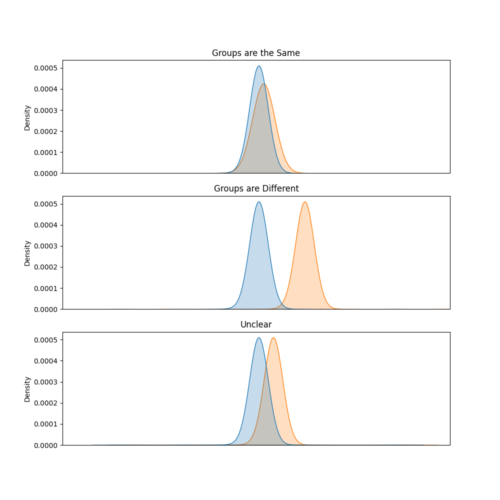
In the baseline case BEST operates by simply fitting distributions over the quantity of interest for every group and then comparing these distributions. Because in the Bayesian paradigm we have entire distributions to work with, instead of singular point estimates, the approach is fundamentally more informative that traditional NHST. In rendering our decision we essentially examine the resulting distributions as follows:

The distribution chosen for the data is the Student T distribution. This distribution is chosen because, while similar to the Normal, it has thicker tails and hence it is better at describing data with “extreme” values, which are quite common in practice. The Student T distribution (in one dimension) is given by:

\[f(x,\mu, \lambda, \nu) = \frac{\Gamma (\frac{\nu+1}2 )}{ \Gamma (\frac \nu 2)} \big( \frac{\lambda}{\pi\nu} \big)^{\frac 12} \big[1+\frac{\lambda (x-\mu)^2}{\nu} \big]^ {-\frac {\nu+1}2 } \]

This distribution is defined by three shape parameters, two which identical to the Normal (mean and standard deviation) and a unique parameter \(\nu\). This parameter is called the degrees of freedom and determines essentially the “normality” of the distribution. For values of \(\nu\) close to 1, the distribution has thick tails, which shrink towards the equivalent normal as it increases.

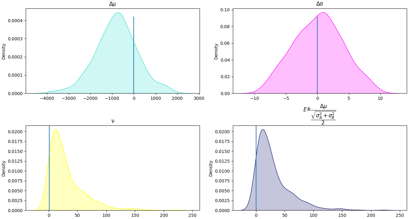
From the above, we can calculate any derived, deterministic quantity, primarily the difference of means (\(\Delta \mu\)), the difference of standard deviations (\(\Delta \sigma\)) This immediately means we receive richly detailed information about the problem at hand, having several distributions to work with rather that simplistic point estimates

Because these are distributions, we can directly interpret them without requiring the convoluted reasoning typing involved in NHSTs. The mode of these distributions is the expected value and the variance can be directly interpreted as the uncertainty. The narrower the distribution is, the more certain we are of the value.

We can also define an additional quantity which Kruschke terms the **effect size**(\(E\)). This is intended to express a kind of standardized effect magnitude, though it is harder to interpret than the rest, since it is not in the original units:

\[E_{ij} \triangleq \dfrac{ \Delta \mu_{ij}}{ \frac{\sqrt{\sigma_i^2+\sigma_j^2}}{2} } \]

\(\Delta\mu\) expresses the expected difference between the groups and hence is the quantity we are primarily interested in. \(\Delta\sigma\) expresses the difference is variances between groups and hence can be interpreted as expressing whether specific instances of the observed, are affected differently for certain values of the grouping variable. The effect size expresses a standardized measure of the “magnitude” of the difference.

Note

The ‘effect size’ quantity is somewhat harder to interpret, because it not in the original units. It is not included by default and has to be explicitly specified by the user as effect_size=True to the BEST model object

We can phrase this problem more abstractly, which will be useful latter when multiple groups will be discussed. Let \(\overset{N \times M+1}{X}\) be a matrix representing our measurements. This matrix is composed of \(N\) observations of \(M\) continuous variables, and we further assume an additional, categorical variable whose values represent the groups themselves. Suppose this group variable takes \(K\) possible values. We split the data according to the value of this variable \({\mathbf{X_0,\dots,X_K}}\) and fit distributions to each group.

We can express this grouping as:

\[\begin{array}{c} \mathbf{X_0} \thicksim \mathcal{T}(\nu_0, \mu_0, \sigma_0)\\ \mathbf{X_1} \thicksim \mathcal{T}(\nu_1, \mu_1, \sigma_1)\\ \vdots\\ \mathbf{X_K} \thicksim \mathcal{T}(\nu_K, \mu_K, \sigma_K)\\ \end{array} \]

We must specify priors for these free parameters, which will be estimated from the observed data. Kruschke proposes the following prior distributions:

\[\begin{array}{c} \nu_0=\nu_1=\dots =\nu_K=\nu\\ \\ \nu \thicksim 1 + \mathcal{Exp}(\lambda=\frac 1 {29.0})\\ \\ \mu_k \thicksim \mathcal{N}(\bar{\mu}_k,\ 2\bar{\sigma_k})\\ \\ \sigma_k \thicksim \mathcal{U}(10^{-3}, 10^3) \end{array} \]

These are rather diffuse priors, placing considerable probability density over a large interval of values. More importantly, they do not favour on group over the over. Graphically we depict these as:

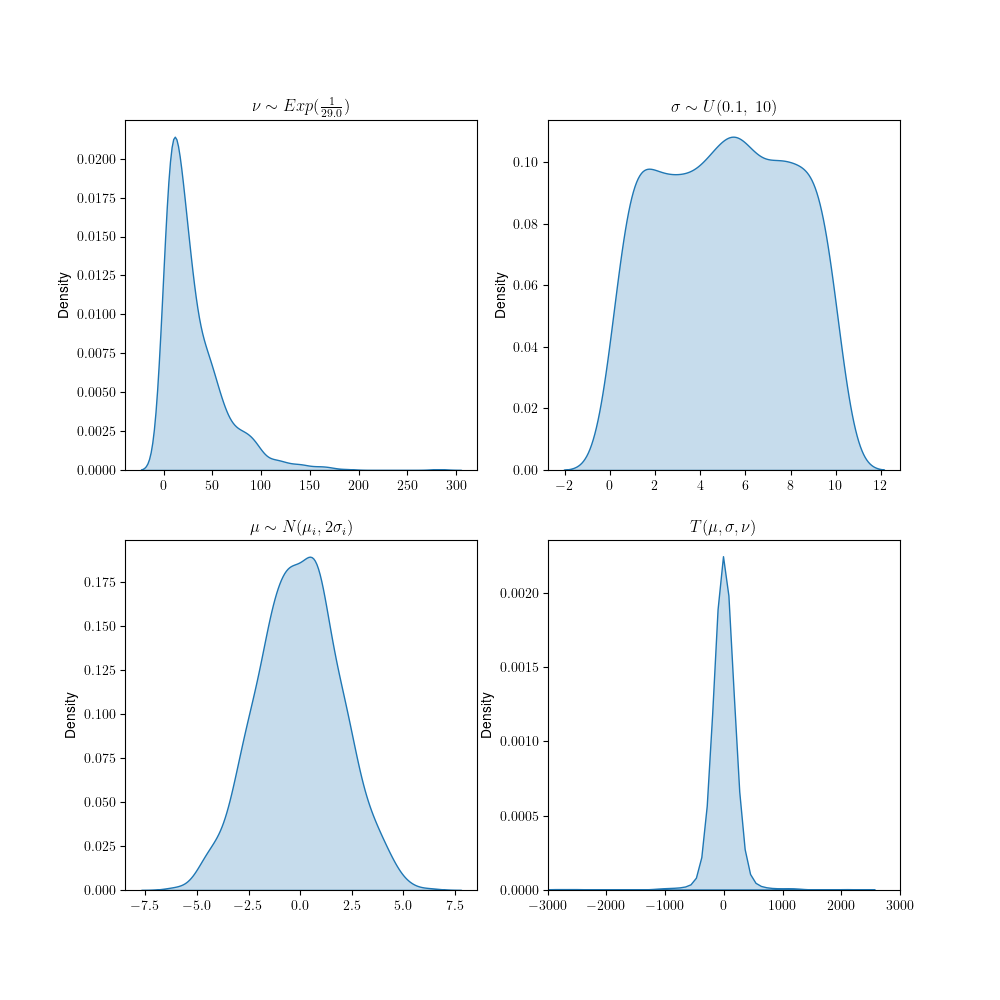
We can make the simplifying assumption that the degrees of freedom are the same across all groups, which is usually a good idea (but not necessary) as we’ve found the alternative usually results in overfitting. For the means, we declare one per group (as per Kruschke’s paper) and set them to a Normal centered around the empirical pooled mean and standard deviation of the group itself. These quantities are derived from the observations themselves, and constitute wide, uninformative priors. More importantly, this does not favor one group over the other a priori. For standard deviations we select a uniform distribution in the interval \([0.0001, 1000]\). As Kruschke himself notes, these priors are exceedingly wide, and described this way only to abstractly encompass all possible data (astronomical, medical, etc). For most real-world applications, they are excessively large and should be adjusted according the data and their units.

Note

The default values for the Uniform distribution are \(0.1-10\) as opposed to \(10^{-3}-10^3\)

Note

bayesian-models assumes the same degrees of freedom across all distributions and uses univariate student T by default. These defaults are chosen because they are quite sensible and closely follow the original formulation. Advanced users are given the option to set independent degrees of freedom for each univariate Student T, or even use a multivariate distribution instead. These settings are not recommended as in our experience allowing different degrees of freedom usually results in over fitting. The multivariate case assumes a diagonal scale matrix is computationally more expensive

Making Decisions:

To move from the hazy space of probabilities to that of actionable decisions, we need to propose, apply and justify a decision rule. Classical hypothesis testing typically justifies its decision making process by appealing to reproducibility. Applying the t-Test is valid, because it ensures Type I and Type II errors are minimized in the long run, for infinite experiments and infinite researchers. There are multiple rules by which one can arrive to binary (or really tertiary) decisions - the one considered here is the earliest proposed for this model and is called the HDI+ROPE rule. The true innovation of this approach is the definition of the ROPE or the Region Of Practical Equivalence. This is a region of values that practically equivalent to zero. Hence the ROPE interval is defined on a problem specific basis - how big enough of difference is big enough? The credible interval (CI) is Bayesian equivalent of the confidence interval and expresses a similar idea. It can be though of as the interval of values considered plausible (under some probability threshold). From these two we can arrive at our decisions according to the following rule:

1. If the CI and the ROPE have nothing in common, then none of the plausible values are equivalent to zero. We therefore decide the groups are different.
2. If the CI is entirely inside the ROPE, then all plausible values are equivalent to zero. Therefore we decide the groups are the same.
3. If the two intervals partially overlap, then some plausible values are equivalent to zero, while some are not. We therefore withhold our decision or simple declare it Indeterminate.

This decision rule can be justified via a branch of mathematics called Bayesian Decision Theory which studies decisions under a state of uncertainty. A full description is outside the scope of this document (and this library), however we can provide a rough outline. We begin by observing that decisions are generally not made in a vacuum but are attended by actions. We therefore denote \(\alpha\in \Alpha\) the set all possible actions, \(\Theta\) the space of all possible values of model parameters and \(\mathcal{X}\) the space of all possible inputs. We define a loss function:

\[L:\mathcal{\Theta}\times\mathcal{\Alpha}\rightarrow \mathbb{R}_0^+ \]

This function maps values of the model and decisions taken to a “cost” of making this decision. We then define a decision function:

\[\delta :\Theta \rightarrow \Alpha \]

From this, justification can be derived in a general way. In practice formulating a problem specific loss function is usually difficult in practice

Extensions:

Multiple Inputs:

To extend the model for multiple inputs, there are several options. We can replace the univariate with a multivariate Student T, or use multiple, univariate distributions. The multivariate Student T has a pdf of:

\[f(\mathbf{x}, \nu,\mu,\Sigma) = \frac{ \Gamma\left[(\nu+p)/2\right]}{ \Gamma(\nu/2)\nu^{p/2}\pi^{p/2 }\left|{\Sigma}\right|^{1/2}\left[1+\frac{1}{\nu}({ \mathbf x}-{\mu})^T{\Sigma}^{-1}({\mathbf x}-{\mu})\right]^{ -(\nu+p)/2} } \]

Note the Multivariate distribution, replaces the parameter \(\sigma\) with a covariance matrix. The element of the diagonal of his matrix are variances across each input variable, and the off-diagonal elements are covariances between different variables. We assume this matrix is diagonal i.e. that there are no covariances between the input variables (since we are generally not interested in describing the covariances themselves). Alternatively we can fit independent univariate distributions for each input variable. We can assume the same degrees of freedom for each of allow them to be independent. The former case is theoretically identical to the multivariate with a diagonal covariance matrix, but more computationally expensive. The latter case is possible but prone to overfitting.

Multiple Groups:

Kruschke provides some guidelines on how to extend this model for multiple groups but provides no tangible examples. We interpret his recommendation to place independent \(\mu_k\) and \(\nu_k\) as pair-wise comparisons between the groups. Hence we implement comparisons for all combinations of values of the grouping variable. Therefore, for \(i,j\in\{0, \dots K\}\) we generate all combinations (unique pairs without repetition or order) and the derived metrics would be:

\[\begin{array}{c} \Delta\mu_{00}\\ \Delta\sigma_{00}\\ E_{00}\\ \Delta\mu_{01}\\ \Delta\sigma_{01}\\ E_{01}\\ \vdots\\ \Delta\mu_{ij}\\ \Delta \sigma_{ij}\\ E_{ij}\\ \vdots\\ \Delta\mu_{KK-1}\\ \Delta \sigma_{KK-1}\\ E_{KK-1}\\ \end{array} \]

Options and Alternative Formulations

There are multiple ways to extend the base model, that Kruchke mentions, not all are accounted for in this implementation. The distribution could be replaced with a LogNormal for special cases, for example. There are alternative ways to generalize the model as well. One could for example relax the diagonality assumption and model the resulting matrices with the specialized LKJCholesky distribution (included in pymc). Another possibility is including a hierarchical distribution for the means, however this formulation is rather nebulous and would likely overcomplicate things. For this reason we chose not to include it. It could potentially be considered in the future however. In terms of the options that are present in this implementation, the default option is univariate distribution with common degrees of freedom. Allowing independent degrees of freedom for input variables, we’ve found (via loo) usually results in overfitting. This case is identical to the multivariate, but more efficient.

Implementation:

The terms of the actual software implementation, the above model is represented by the bayesian_models.models.BEST class. Like all models it implements the general four methods __init__, __call__, fit and predict. The __init__ method is responsible of setting all parameters and hyperparameters of the model itself. Unusually, these are class methods rather than object methods. This choice was made to enable rapid prototyping as the expected use-case is that a single ‘version’ of the model can be applied to multiple data (multiple variables to group by), because we often deal with datasets with multiple categorical variables and we are interested in knowing whether these variables impact other continuous variables. This model accepts no “testing” data, and hence its data containers are declared immutable. The predict method itself renders the decisions and returns findings as a dictionary, mapping each quantity \(\Delta \mu_{ij}\), \(\Delta \sigma_{ij}\), etc to a pandas.DataFrame containing the results. These are typically of the same shape as those of arviz.summary with an additional column representing the decision, according to the HDI+ROPE rule. Other rules are possible, but they are not implemented at present, as we think this rule is very intuitive, easy to use and works well for many common cases. The decision making process itself is deferred to the predict method, since it is meaningless prior to training completion. This way, a user could also rapidly test many options of ROPEs and HDI thresholds on the same model and aggregate the results, without retraining each time. After all the decision making process itself is independent of the inference process.